Graph-based Intrusion Detection

Security

Intrusion

Analysis

torch-geometric KGNN for Intrusion Detection and explanation

Published

May 6, 2025

Canadian Institute for Cybersecurity CIC-IDS2017

The IDS dataset is an evaluation of Intrusion Detection Systems.

I will be transposing this into into a graph data structure in order to temporally evaluate relationships between features (edges). Then a GraphNeuralNet model will be trained to determine which type of intrusion is happening by reading the parameters of the network. Finally I will briefly touch on creating an interactive explanation of nodes with torch_geometric.

This notebook was run on Hugging Face Spaces, JupyterLab using L40S.

!pip install torch torch_geometric polars seaborn scikit-learn

import polars as pl
import numpy as np
import torch
from torch_geometric.data import Data
from sklearn.preprocessing import LabelEncoder, StandardScaler

#The dataset be a concatenation of the following files
files = [
    'Monday-WorkingHours.pcap_ISCX.csv',
    'Tuesday-WorkingHours.pcap_ISCX.csv',
    'Wednesday-workingHours.pcap_ISCX.csv',
    'Thursday-WorkingHours-Morning-WebAttacks.pcap_ISCX.csv',
    'Thursday-WorkingHours-Afternoon-Infilteration.pcap_ISCX.csv',
    'Friday-WorkingHours-Morning.pcap_ISCX.csv',
    'Friday-WorkingHours-Afternoon-PortScan.pcap_ISCX.csv',
    'Friday-WorkingHours-Afternoon-DDos.pcap_ISCX.csv'
]

dfs = [pl.read_csv(file, 
                   infer_schema_length=10000, 
                   null_values=['Infinity', "NaN"]) for file in files]
full_df = pl.concat(dfs)

# Remove leading spaces from columns
full_df = full_df.rename({col: col.strip() for col in full_df.columns})
full_df = full_df.fill_nan(None).drop_nulls()

# Basic preprocessing
label_encoder = LabelEncoder()
y_encoded = label_encoder.fit_transform(full_df["Label"])

print("Label mapping:", pl.DataFrame(dict(zip(label_encoder.classes_, label_encoder.transform(label_encoder.classes_)))))

Y = torch.tensor(y_encoded, dtype=torch.long) # converting to torch within numpy accelerates the tensor transformation

features = [
    'Destination Port', 'Flow Duration', 'Total Fwd Packets',
    'Total Backward Packets', 'Total Length of Fwd Packets', 'Total Length of Bwd Packets',
    'Fwd Packet Length Max', 'Fwd Packet Length Min', 'Fwd Packet Length Mean',
    'Fwd Packet Length Std', 'Bwd Packet Length Max', 'Bwd Packet Length Min',
    'Bwd Packet Length Mean', 'Bwd Packet Length Std', 'Flow Bytes/s',
    'Flow Packets/s', 'Flow IAT Mean', 'Flow IAT Std',
    'Flow IAT Max', 'Flow IAT Min', 'Fwd IAT Total',
    'Fwd IAT Mean', 'Fwd IAT Std', 'Fwd IAT Max',
    'Fwd IAT Min', 'Bwd IAT Total', 'Bwd IAT Mean',
    'Bwd IAT Std', 'Bwd IAT Max', 'Bwd IAT Min',
    'Fwd PSH Flags', 'Bwd PSH Flags', 'Fwd URG Flags',
    'Bwd URG Flags', 'Fwd Header Length', 'Bwd Header Length',
    'Fwd Packets/s', 'Bwd Packets/s', 'Min Packet Length',
    'Max Packet Length', 'Packet Length Mean', 'Packet Length Std',
    'Packet Length Variance', 'FIN Flag Count', 'SYN Flag Count',
    'RST Flag Count', 'PSH Flag Count', 'ACK Flag Count',
    'URG Flag Count', 'CWE Flag Count', 'ECE Flag Count',
    'Down/Up Ratio', 'Average Packet Size', 'Avg Fwd Segment Size',
    'Avg Bwd Segment Size', 'Fwd Avg Bytes/Bulk', 'Fwd Avg Packets/Bulk',
    'Fwd Avg Bulk Rate', 'Bwd Avg Bytes/Bulk', 'Bwd Avg Packets/Bulk',
    'Bwd Avg Bulk Rate', 'Subflow Fwd Packets', 'Subflow Fwd Bytes',
    'Subflow Bwd Packets', 'Subflow Bwd Bytes', 'Init_Win_bytes_forward',
    'Init_Win_bytes_backward', 'act_data_pkt_fwd', 'min_seg_size_forward',
    'Active Mean', 'Active Std', 'Active Max',
    'Active Min', 'Idle Mean', 'Idle Std',
    'Idle Max', 'Idle Min'
]
X_np = full_df.select(features).to_numpy()
scaler = StandardScaler()
X_scaled = scaler.fit_transform(X_np)

X = torch.tensor(X_scaled, dtype=torch.float32)

del X_np, y_encoded, scaler, X_scaled
# Remember to check for open Python processes after finished with the notebook.

Label mapping: shape: (1, 15)
┌────────┬─────┬──────┬──────────────┬───┬─────────────┬──────────────┬──────────────┬─────────────┐
│ BENIGN ┆ Bot ┆ DDoS ┆ DoS          ┆ … ┆ SSH-Patator ┆ Web Attack � ┆ Web Attack � ┆ Web Attack  │
│ ---    ┆ --- ┆ ---  ┆ GoldenEye    ┆   ┆ ---         ┆ Brute Force  ┆ Sql          ┆ � XSS       │
│ i64    ┆ i64 ┆ i64  ┆ ---          ┆   ┆ i64         ┆ ---          ┆ Injection    ┆ ---         │
│        ┆     ┆      ┆ i64          ┆   ┆             ┆ i64          ┆ ---          ┆ i64         │
│        ┆     ┆      ┆              ┆   ┆             ┆              ┆ i64          ┆             │
╞════════╪═════╪══════╪══════════════╪═══╪═════════════╪══════════════╪══════════════╪═════════════╡
│ 0      ┆ 1   ┆ 2    ┆ 3            ┆ … ┆ 11          ┆ 12           ┆ 13           ┆ 14          │
└────────┴─────┴──────┴──────────────┴───┴─────────────┴──────────────┴──────────────┴─────────────┘

# KNN graph creation
from sklearn.neighbors import kneighbors_graph
from sklearn.model_selection import train_test_split
import os

# check if intrusion_graph.pt already exists
if os.path.exists('intrusion_graph.pt'):
    print("Loading existing graph...")
    data = torch.load('intrusion_graph.pt', weights_only=False)
else:
    # Create KNN graph based on feature similarity
    adj = kneighbors_graph(X, n_neighbors=5, mode='connectivity', include_self=False, n_jobs=-1) # using all cores requires more work
    edge_index = torch.tensor(np.array(adj.nonzero()), dtype=torch.long)

    # Create PyG Data object
    data = Data(x=X, edge_index=edge_index, y=Y)
    
    # Save because this took 2.5 hours.
    torch.save(data, 'intrusion_graph.pt') # PyTorch Binary

# Train/test split (stratified by label)
train_mask = torch.zeros(len(Y), dtype=torch.bool)
test_mask = torch.zeros(len(Y), dtype=torch.bool)

indices = np.arange(len(Y))
train_idx, test_idx = train_test_split(indices, test_size=0.3, 
                                     stratify=Y, random_state=123)

train_mask[train_idx] = True
test_mask[test_idx] = True

data.train_mask = train_mask
data.test_mask = test_mask

Loading existing graph...

# Destination Port Graph

# Create nodes based on destination ports
port_features = (
    full_df.group_by("Destination Port")
    .agg([
        # For each feature, create mean and std
        *[pl.col(feat).mean().alias(f"{feat}_mean") for feat in features], 
        *[pl.col(feat).std().alias(f"{feat}_std") for feat in features]
    ])
)

# Get unique ports and create mapping
unique_ports = port_features["Destination Port"].to_list()
port_to_idx = {port: idx for idx, port in enumerate(unique_ports)}

x_port = torch.tensor(port_features.drop("Destination Port").to_numpy(), dtype=torch.float32)

# Create edges on sequence of connections
edge_list = []
prev_port = None
for port in full_df["Destination Port"].to_list():
    if prev_port is not None and port != prev_port:
        src = port_to_idx[prev_port]
        dst = port_to_idx[port]
        edge_list.append((src, dst))
    prev_port = port

edge_index = torch.tensor(edge_list).t().contiguous() if edge_list else torch.empty((2, 0), dtype=torch.long)

# Create labels (most common label per port)  # Doesn't work well for common ports which is why this was abandoned for time being
port_labels = (
    full_df.group_by("Destination Port")
    .agg(pl.col("Label").mode().first())
    .sort("Destination Port")
    .select("Label")
    .to_series()
    .to_numpy()
)

y_port = torch.tensor(label_encoder.transform(port_labels), dtype=torch.long)

data_port = Data(x=x_port, edge_index=edge_index, y=y_port)

def print_graph_stats(data):
    print(f"Number of nodes: {data.num_nodes:,}")
    print(f"Number of edges: {data.num_edges:,}")
    print(f"Average node degree: {data.num_edges / data.num_nodes:.2f}")
    print(f"Number of node features: {data.num_node_features}")
    print(f"Number of classes: {len(torch.unique(data.y))}")
    
    # Label distribution
    unique, counts = torch.unique(data.y, return_counts=True)
    print("\nLabel distribution:")
    for u, c in zip(unique, counts):
        print(f"Class {u.item()}: {c.item():,} ({c.item()/data.num_nodes:.1%})")

print_graph_stats(data)

Number of nodes: 2,827,876
Number of edges: 14,139,380
Average node degree: 5.00
Number of node features: 77
Number of classes: 15

Label distribution:
Class 0: 2,271,320 (80.3%)
Class 1: 1,956 (0.1%)
Class 2: 128,025 (4.5%)
Class 3: 10,293 (0.4%)
Class 4: 230,124 (8.1%)
Class 5: 5,499 (0.2%)
Class 6: 5,796 (0.2%)
Class 7: 7,935 (0.3%)
Class 8: 11 (0.0%)
Class 9: 36 (0.0%)
Class 10: 158,804 (5.6%)
Class 11: 5,897 (0.2%)
Class 12: 1,507 (0.1%)
Class 13: 21 (0.0%)
Class 14: 652 (0.0%)

import matplotlib.pyplot as plt
import seaborn as sns

def plot_feature_distribution(data, feature_index):
    plt.figure(figsize=(12, 6))
    plt.hist(data.x[:, feature_index].numpy(), bins=50, color="darkred", alpha=0.7)
    plt.xlabel(f"Feature {feature_index}")
    plt.ylabel("Frequency")
    plt.title(f"Distribution of Feature {feature_index}")
    plt.show()

plot_feature_distribution(data, 0)  # Can be run for all classes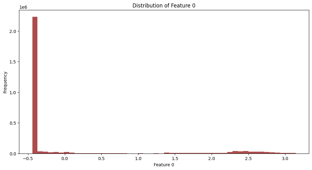

from collections import Counter

label_counts = Counter(data.y.numpy())
total = sum(label_counts.values())
label_percents = {k: v/total*100 for k, v in label_counts.items()}

plt.figure(figsize=(12, 6))
sns.barplot(x=list(label_percents.keys()), 
            y=list(label_percents.values()), color='darkred')
plt.title("Attack Type Distribution (%)")
plt.xlabel("Label Class")
plt.ylabel("Percentage")
plt.xticks(rotation=45, ticks=list(label_percents.keys()), labels=label_encoder.inverse_transform(list(label_percents.keys())))
plt.show()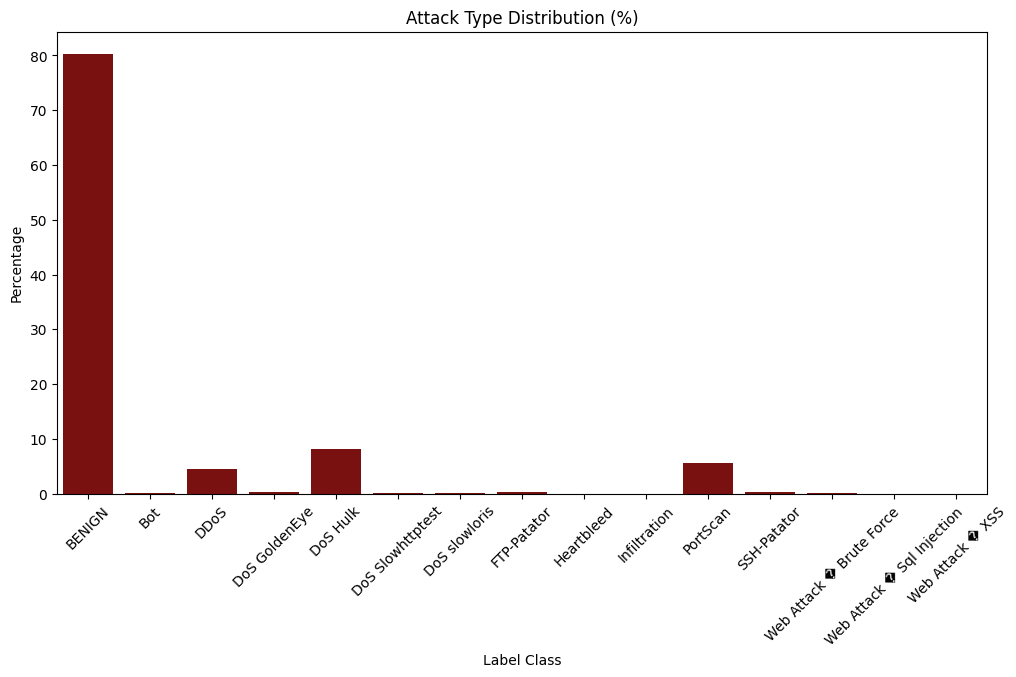

import pandas as pd

def analyze_neighborhoods(data, num_samples=5):
    results = []
    for label in torch.unique(data.y):
        label_nodes = (data.y == label).nonzero().squeeze()
        sampled_nodes = label_nodes[torch.randperm(len(label_nodes))[:num_samples]]
        
        for node in sampled_nodes:
            neighbors = data.edge_index[1][data.edge_index[0] == node]
            neighbor_labels = data.y[neighbors]
            
            # Calculate label distribution in neighborhood
            unique, counts = torch.unique(neighbor_labels, return_counts=True)
            results.append({
                'center_label': label.item(),
                'neighbor_labels': dict(zip(unique.tolist(), counts.tolist()))
            })
    
    return pd.DataFrame(results)

neighbor_stats = analyze_neighborhoods(data)
print(neighbor_stats.groupby('center_label').describe())

             neighbor_labels                            
                       count unique             top freq
center_label                                            
0                          5      1          {0: 5}    5
1                          5      3    {0: 2, 1: 3}    3
2                          5      1          {2: 5}    5
3                          5      1          {3: 5}    5
4                          5      1          {4: 5}    5
5                          5      1          {5: 5}    5
6                          5      1          {6: 5}    5
7                          5      1          {7: 5}    5
8                          5      1          {8: 5}    5
9                          5      3    {0: 2, 9: 3}    2
10                         5      3         {10: 5}    3
11                         5      1         {11: 5}    5
12                         5      3  {12: 4, 14: 1}    3
13                         5      5   {0: 1, 11: 4}    1
14                         5      4  {12: 3, 14: 2}    2

from torch_geometric.explain import Explainer # https://pytorch-geometric.readthedocs.io/en/2.6.0/modules/explain.html
from torch_geometric.nn import GCNConv, SAGEConv #https://www.reddit.com/r/learnmachinelearning/comments/1dsvamf/what_is_the_difference_between_graph_convolution/
from torch_geometric.explain import GNNExplainer
import torch.nn.functional as F

class IntrusionGNN(torch.nn.Module):
    def __init__(self, in_channels, hidden_channels, out_channels):
        super().__init__()
        self.conv1 = SAGEConv(in_channels, hidden_channels)
        self.conv2 = SAGEConv(hidden_channels, out_channels)
        
    def forward(self, x, edge_index):
        x = self.conv1(x, edge_index).relu()
        x = F.dropout(x, p=0.5, training=self.training)
        return self.conv2(x, edge_index)
    
device = torch.device('cuda' if torch.cuda.is_available() else 'cpu')
print(f"Using device: {device}")

model = IntrusionGNN(in_channels=data.num_features, 
                     hidden_channels=64, 
                     out_channels=len(torch.unique(data.y))).to(device)

data.to(device)

explainer = Explainer(
    model=model,
    algorithm=GNNExplainer(epochs=200),
    explanation_type='model',
    node_mask_type='attributes',
    edge_mask_type='object',
    model_config=dict(
        mode='multiclass_classification',
        task_level='node',
        return_type='log_probs'
    )
)

optimizer = torch.optim.Adam(model.parameters(), lr=0.01)
criterion = torch.nn.CrossEntropyLoss()

def train():
    model.train()
    optimizer.zero_grad()
    out = model(data.x, data.edge_index)
    loss = criterion(out[data.train_mask], data.y[data.train_mask])
    loss.backward()
    optimizer.step()
    return loss.item()

for epoch in range(1, 301):
    loss = train()
    if epoch % 10 == 0:
        print(f'Epoch: {epoch:03d}, Loss: {loss:.4f}')

You may be wondering what the next cell actually shows us, and what we have been making this whole time. The next cell shows us our model's training results as measured in terms of incorrect predictions.

On the 300th epoch of training our model was able to 93% accurately predict which type of intrusion is happening based on unlabled incoming data.

This means our model not only detects an intrusion, but correctly identifies the type as well.

Using device: cuda
Epoch: 010, Loss: 0.4410
Epoch: 020, Loss: 0.2906
Epoch: 030, Loss: 0.2222
Epoch: 040, Loss: 0.1839
Epoch: 050, Loss: 0.1609
Epoch: 060, Loss: 0.1455
Epoch: 070, Loss: 0.1341
Epoch: 080, Loss: 0.1258
Epoch: 090, Loss: 0.1187
Epoch: 100, Loss: 0.1134
Epoch: 110, Loss: 0.1084
Epoch: 120, Loss: 0.1044
Epoch: 130, Loss: 0.1008
Epoch: 140, Loss: 0.0973
Epoch: 150, Loss: 0.0952
Epoch: 160, Loss: 0.0924
Epoch: 170, Loss: 0.0901
Epoch: 180, Loss: 0.0881
Epoch: 190, Loss: 0.0861
Epoch: 200, Loss: 0.0845
Epoch: 210, Loss: 0.0826
Epoch: 220, Loss: 0.0812
Epoch: 230, Loss: 0.0792
Epoch: 240, Loss: 0.0782
Epoch: 250, Loss: 0.0768
Epoch: 260, Loss: 0.0757
Epoch: 270, Loss: 0.0743
Epoch: 280, Loss: 0.0727
Epoch: 290, Loss: 0.0719
Epoch: 300, Loss: 0.0708

def explain_node(node_idx, target_label=None):
    torch.cuda.empty_cache()
    
    explanation = explainer(
        data.x, 
        data.edge_index, 
        index=node_idx)
    
    if hasattr(explanation, 'node_mask'):
        feat_importance = explanation.node_mask.sum(dim=0) if explanation.node_mask.dim() > 1 else explanation.node_mask
    else:
        feat_importance = explanation.node_feat_mask.sum(dim=0)
        
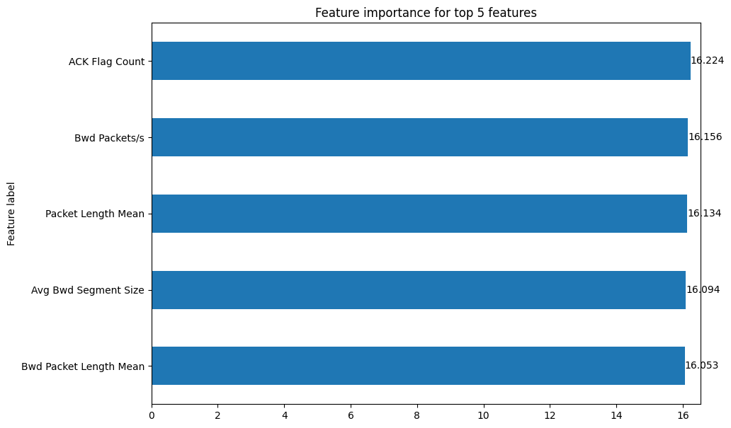
    top_feats = torch.topk(feat_importance, k=5)
    
    print(f"\nExplanation for node {node_idx} (true class: {data.y[node_idx].item()})")
    print("Top important features:")
    for feat_idx, importance in zip(top_feats.indices, top_feats.values):
        print(f"{features[feat_idx]}: {importance:.4f}")
    
    if hasattr(explanation, 'visualize_feature_importance'):
        explanation.visualize_feature_importance(feat_labels=features, top_k=5)
    else:
        plt.figure(figsize=(10, 5))
        plt.barh([features[i] for i in top_feats.indices], top_feats.values.numpy(), color = "darkred")
        plt.title("Feature Importance for Prediction")
        plt.show()

    return explanation

# example usage on node, any node can be set in application.
explain_node(node_idx=123, target_label=None)
explain_node(node_idx=1234, target_label=1)


Explanation for node 123 (true class: 0)
Top important features:
ACK Flag Count: 16.2245
Bwd Packets/s: 16.1562
Packet Length Mean: 16.1341
Avg Bwd Segment Size: 16.0938
Bwd Packet Length Mean: 16.0528